25:00
Presentation ready
plots I:
Telling a story
Lecture 9
Keep it simple
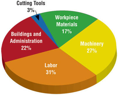
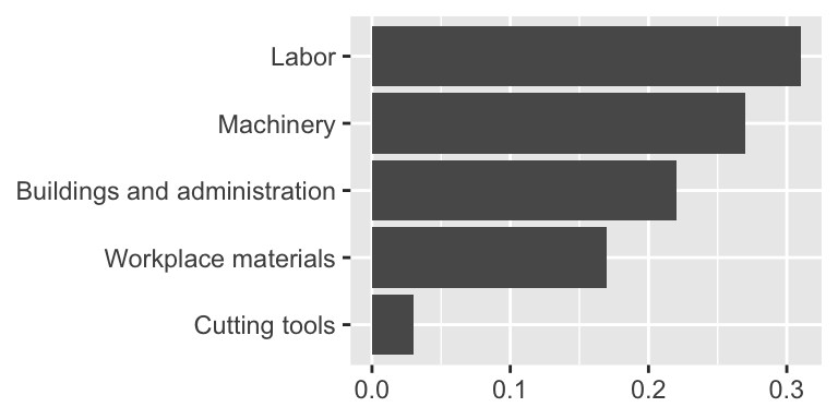
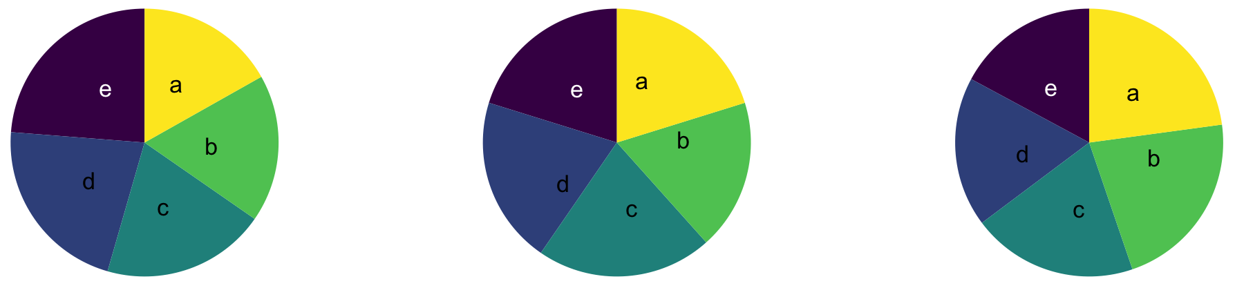
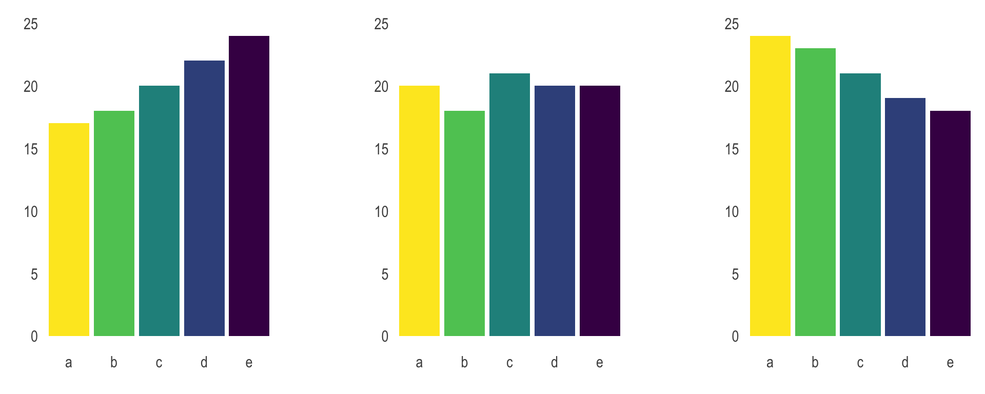
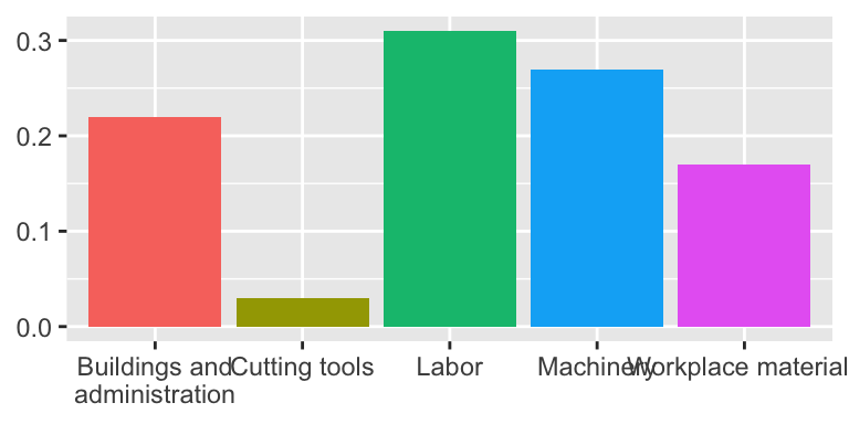
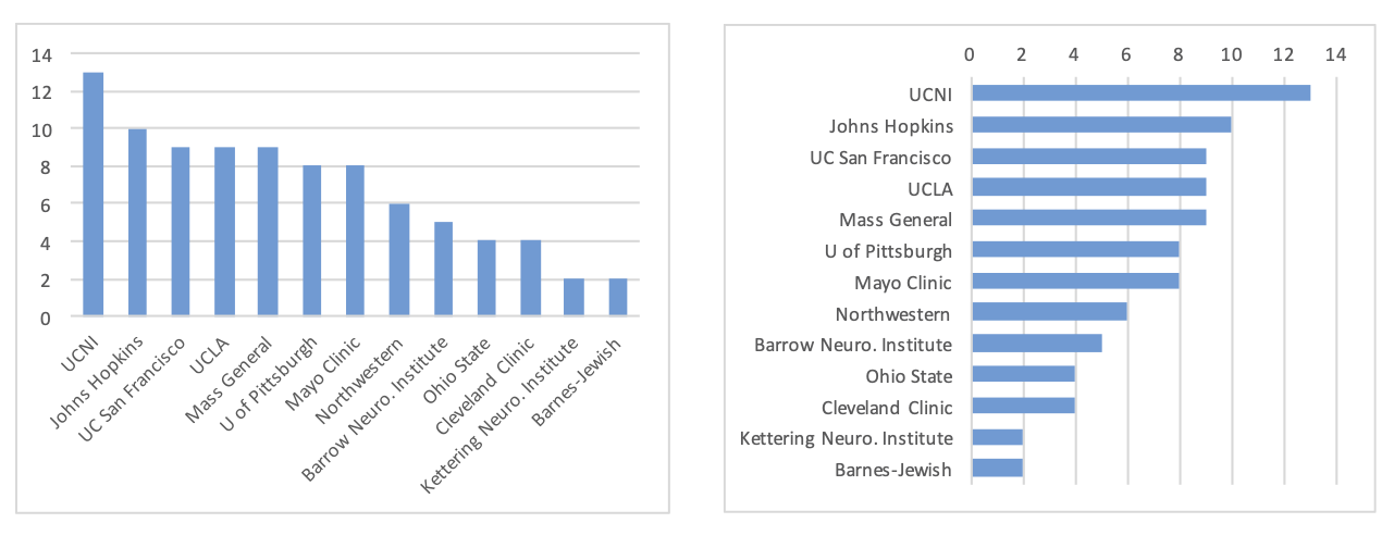
Judging relative area
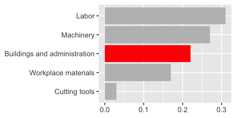
Use color to draw attention
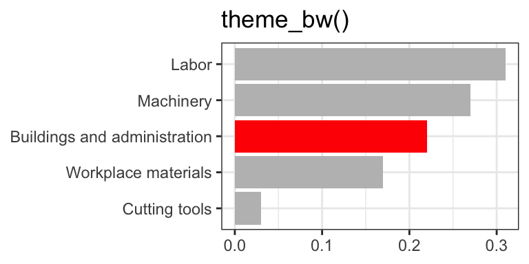
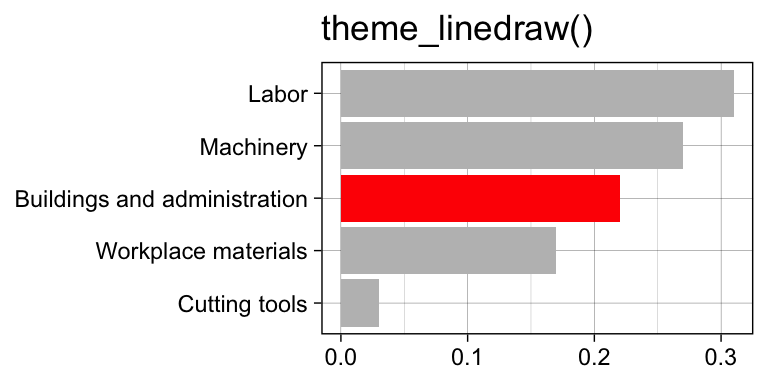
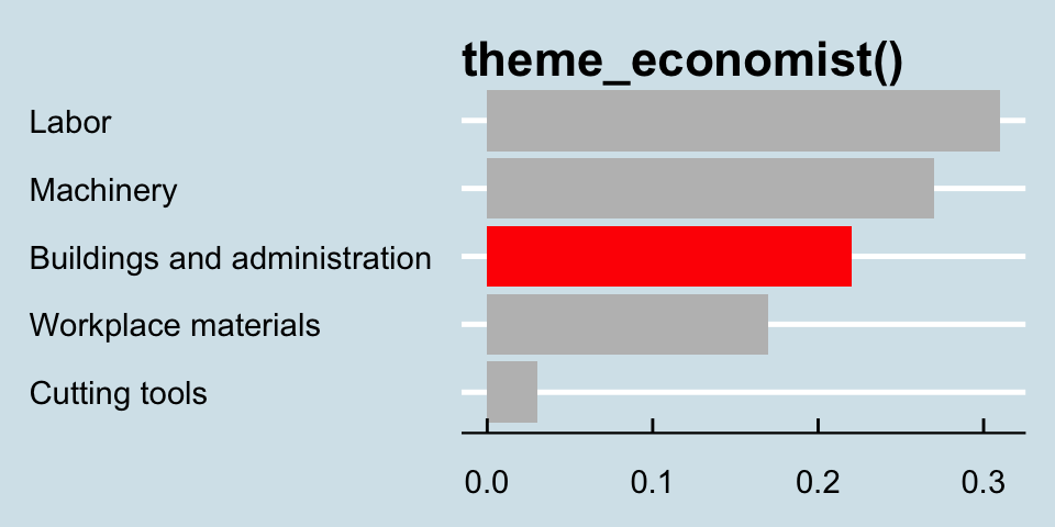
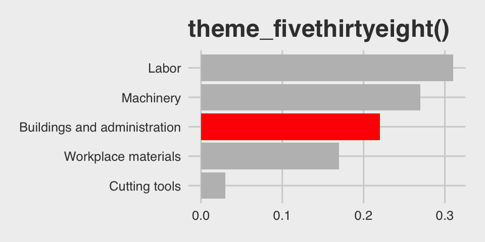
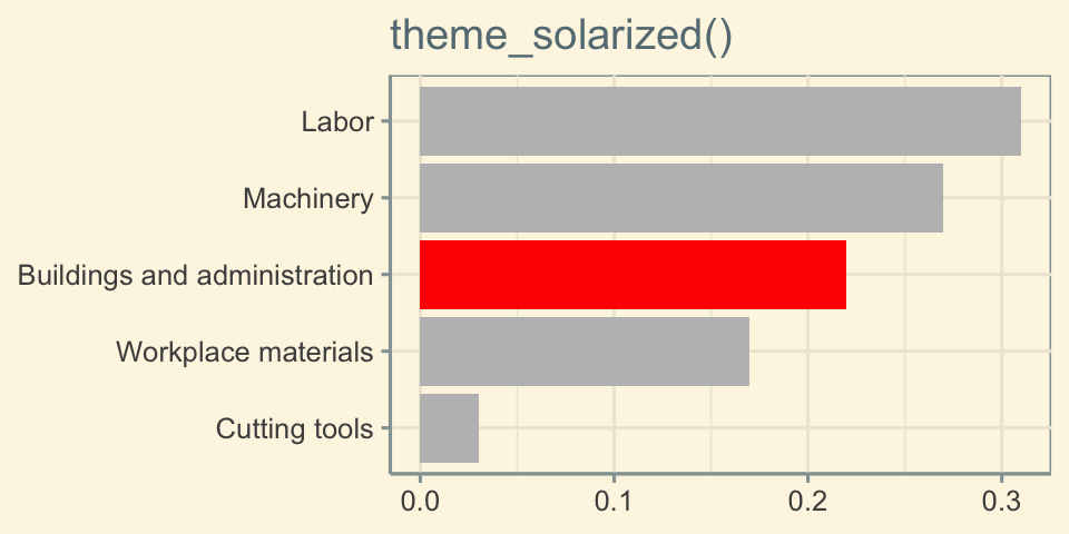
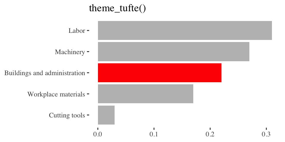
Play with themes for a non-standard look
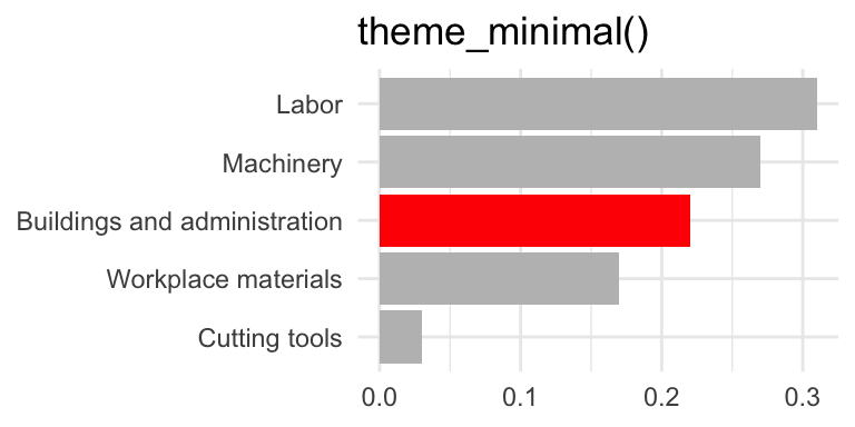
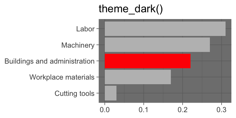
Go beyond ggplot2 themes – ggthemes
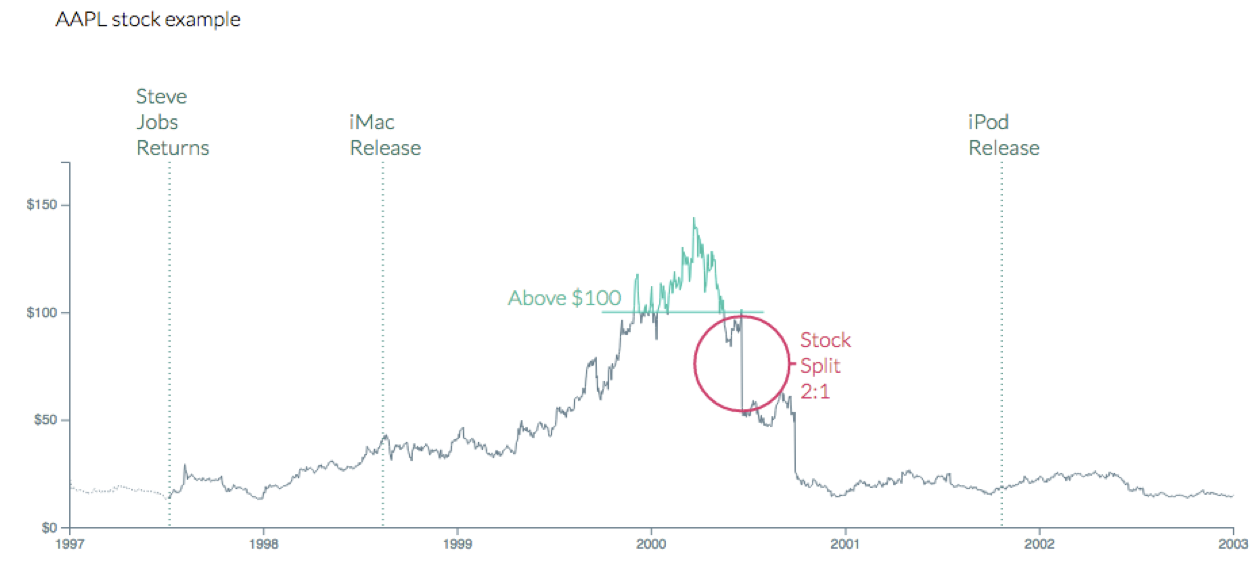
Tell a story
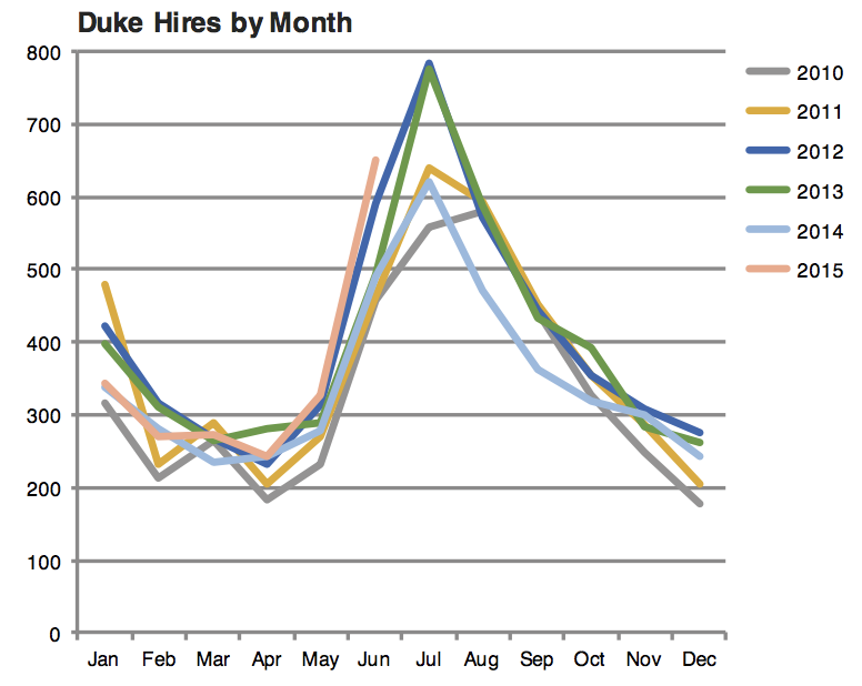
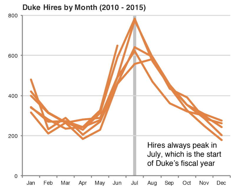
Leave out non-story details
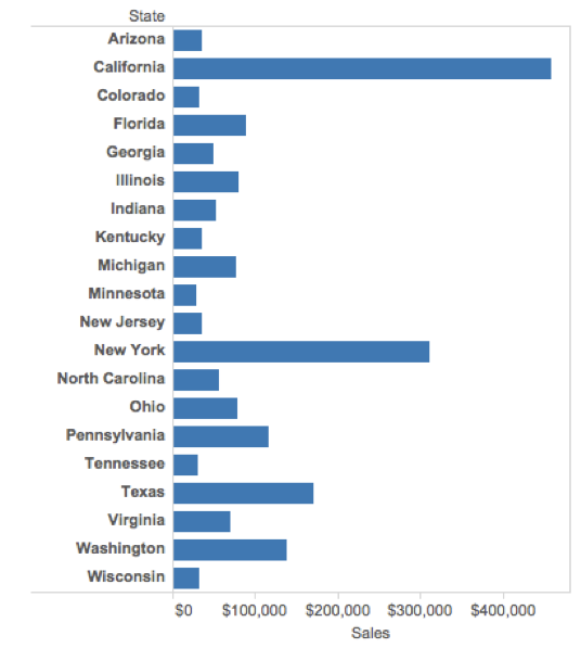
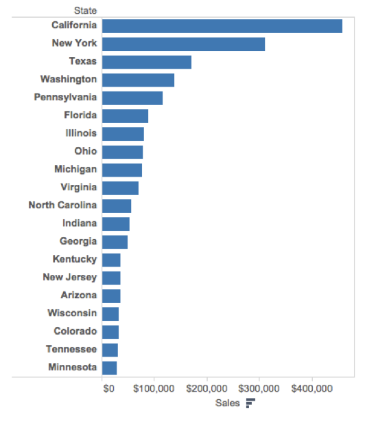
Order matters
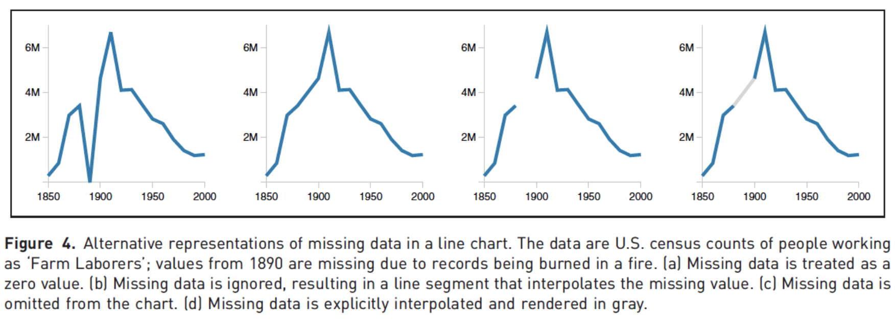
Clearly indicate missing data
Reduce cognitive load
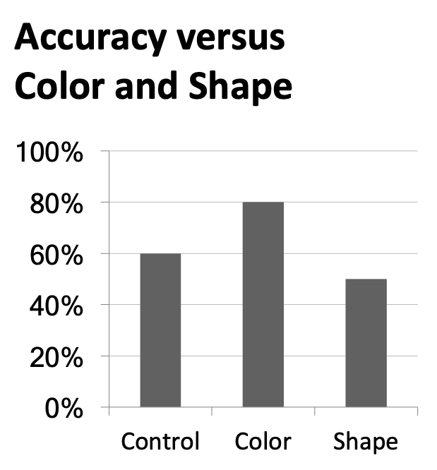
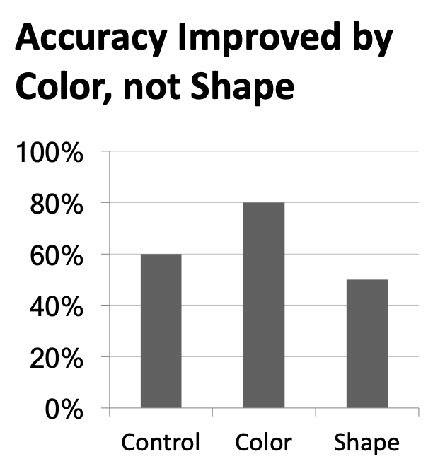
Use descriptive titles
Annotate figures
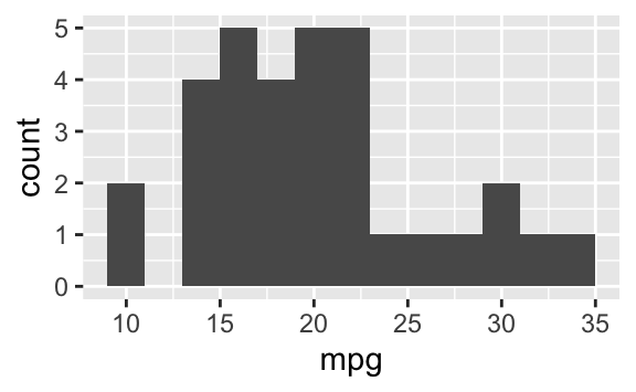
Small fig-width
For a zoomed-in look
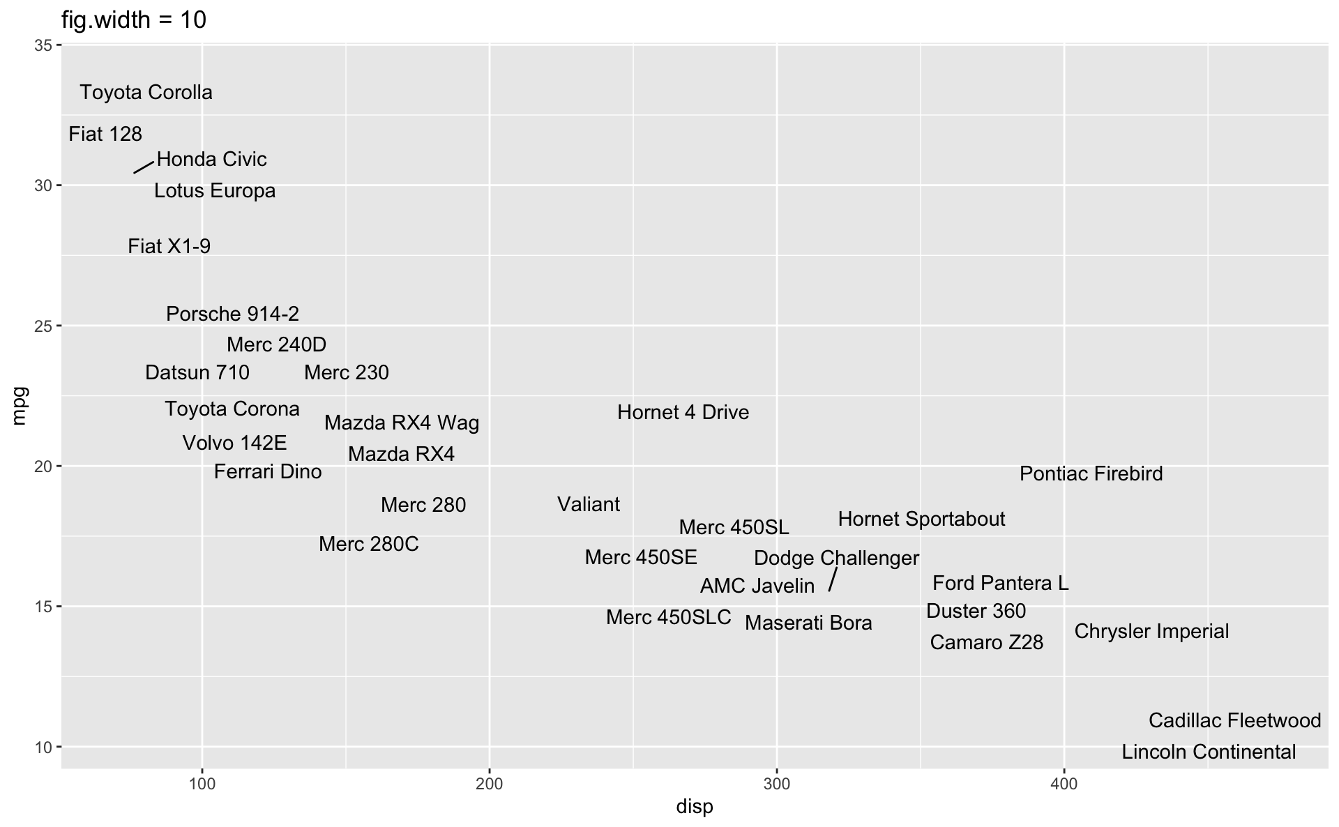
Large fig-width
For a zoomed-out look
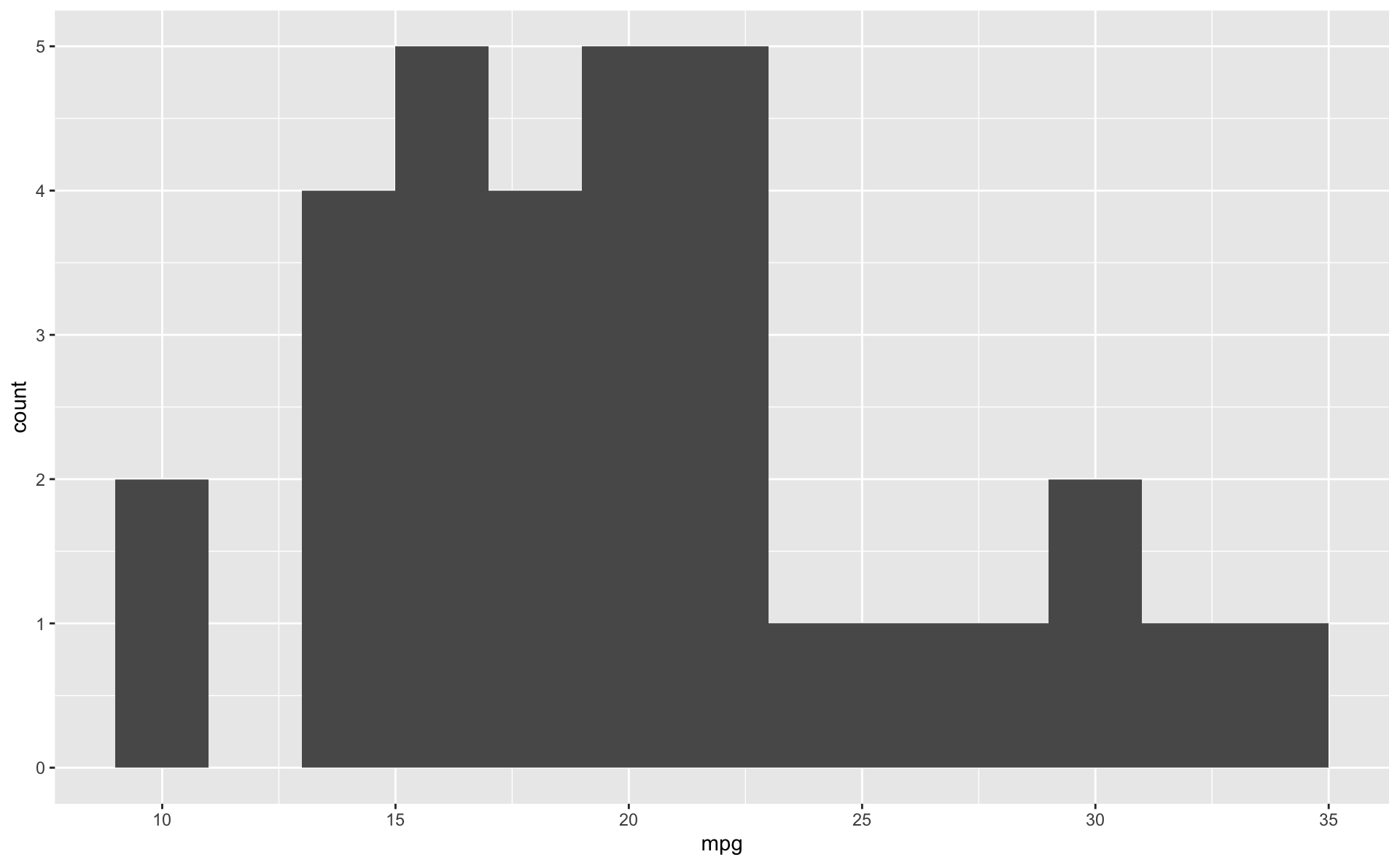
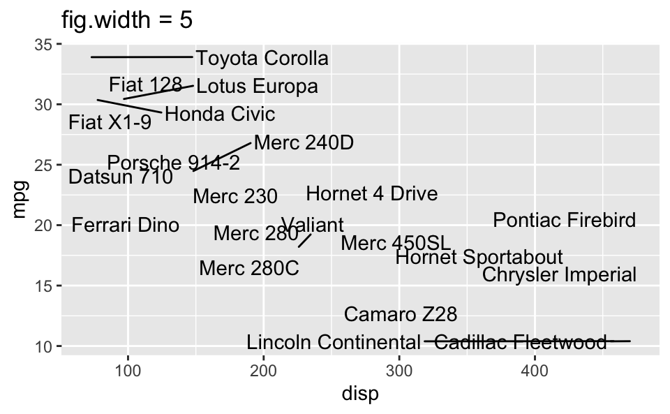
fig-width affects text size
Take home exam redo (optional)
- Due: Friday, Oct 13 at 1 pm
- Must request opening your exam repo back up for resubmission by end of class on Thursday by messaging me on Slack
- Work in
exam-1-redo.qmd, this is a copy of your exam submission, without any changes I might have implemented to get it to render – do not overwriteexam-1.qmd. - Improve your answers working on your own. The same rules as the exam applies.
- You will be eligible to receive up to 50% of the points you missed on the take home portion of the exam.
- There is no in-class exam redo.