Visualizing and modeling relationships III

Lecture 12

Dr. Mine Çetinkaya-Rundel

Duke University
STA 113 - Fall 2023

Warm-up

Announcements

• HW 4 due next Thursday
• OH by appointment this week
• Thursday lecture on Zoom - link to be posted as Canvas announcement and on Slack

Today’s goals

• Fit and interpret models for predicting (classifying) binary outcomes

• Define sensitivity, specificity, and ROC curves

• Visualize decision boundaries for classification models

Logistic regression

So far in regression

• Outcome: Numerical, Predictor: One numerical or one categorical with only two levels \(\rightarrow\) Simple linear regression

• Outcome: Numerical, Predictors: Any number of numerical or categorical variables with any number of levels \(\rightarrow\) Multiple linear regression

• Outcome: Categorical with only two levels, Predictors: Any number of numerical or categorical variables with any number of levels \(\rightarrow\) Logistic regression

• Outcome: Categorical with any number of levels, Predictors: Any number of numerical or categorical variables with any number of levels \(\rightarrow\) Generalized linear models – Not covered in STA 113FS

Data + packages

library(tidyverse)
library(tidymodels)

hp_spam <- read_csv("data/hp-spam.csv")

• 4601 emails collected at Hewlett-Packard labs and contains 58 variables

• Outcome: type

  • type = 1 is spam

  • type = 0 is non-spam

• Predictors of interest:

  • capitalTotal: Number of capital letters in email

  • Percentages are calculated as (100 * number of times the WORD appears in the e-mail) / total number of words in email

    • george: Percentage of “george”s in email (these were George’s emails)

    • you: Percentage of “you”s in email

Glimpse at data

What type of data is type? What type should it be in order to use logistic regression?

hp_spam |>
  select(type, george, capitalTotal, you)

# A tibble: 4,601 × 4
    type george capitalTotal   you
   <dbl>  <dbl>        <dbl> <dbl>
 1     1      0          278  1.93
 2     1      0         1028  3.47
 3     1      0         2259  1.36
 4     1      0          191  3.18
 5     1      0          191  3.18
 6     1      0           54  0   
 7     1      0          112  3.85
 8     1      0           49  0   
 9     1      0         1257  1.23
10     1      0          749  1.67
# ℹ 4,591 more rows

EDA: How much spam?

hp_spam |>
  count(type) |>
  mutate(p = n / sum(n))

# A tibble: 2 × 3
   type     n     p
  <dbl> <int> <dbl>
1     0  2788 0.606
2     1  1813 0.394

EDA: AM I SCREAMING? capitalTotal

ggplot(hp_spam, aes(x = capitalTotal)) +
  geom_histogram()

`stat_bin()` using `bins = 30`. Pick better value with `binwidth`.

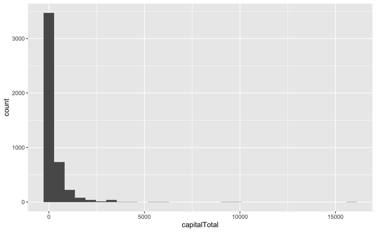
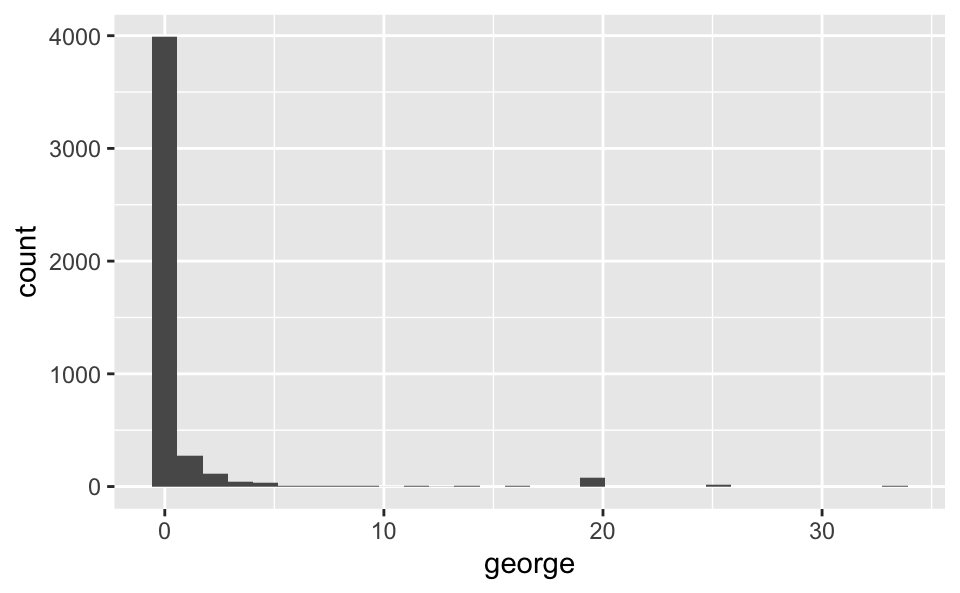
EDA: george, is that you?

ggplot(hp_spam, aes(x = george)) +
  geom_histogram()

`stat_bin()` using `bins = 30`. Pick better value with `binwidth`.

ggplot(hp_spam, aes(x = you)) +
  geom_histogram()

`stat_bin()` using `bins = 30`. Pick better value with `binwidth`.

Logistic regression

• Logistic regression takes in a number of predictors and outputs the probability of a “success” (an outcome of 1) in a binary outcome variable.

• The probability is related to the predictors via a link function,

\[ p(y_i = 1) = \frac{1}{1+\text{exp}({- \sum \beta_i x_i })}, \] whose output is in \((0,1)\) (a probability).

• In this modeling scheme, one typically finds \(\hat{\beta}\) by maximizing the likelihood function, another objective function, different than our previous “least squares” objective.

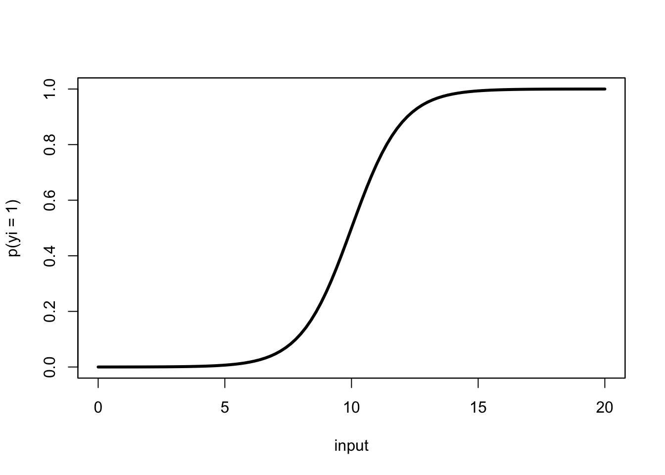
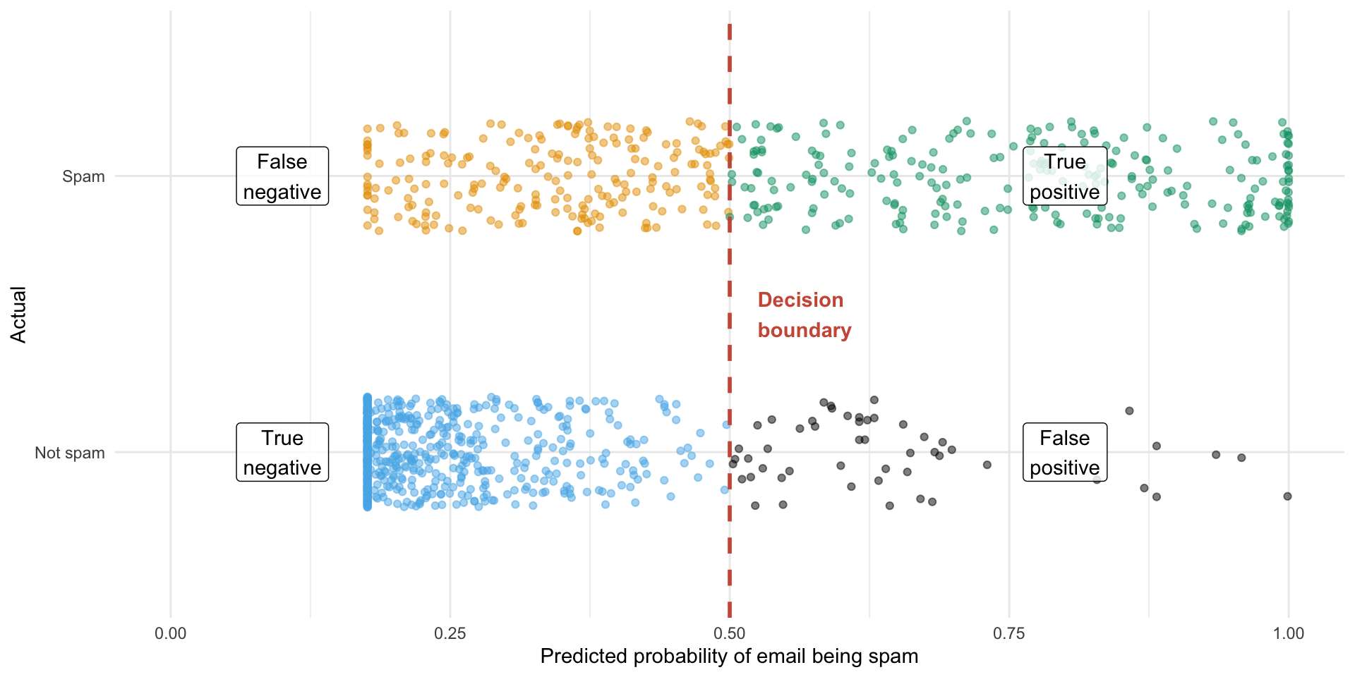
Logistic regression, visualized

Using data to estimate \(\beta_i\)

To proceed with building our email classifier, we will, as usual, use our data (outcome \(y_i\) and predictor \(x_i\) pairs), to estimate \(\beta\) (find \(\hat{\beta}\)) and obtain the model:

\[ p(y_i = 1) = \frac{1}{1+\text{exp}({- \sum \hat{\beta}_i x_i})}, \]

ae-11-spam

Ultimate goal: Recreate the following visualization.

ae-11-spam

Reminder of instructions for getting started with application exercises:

• Go to the course GitHub org and find your ae-11-spam (repo name will be suffixed with your GitHub name).
• Click on the green CODE button, select Use SSH (this might already be selected by default, and if it is, you’ll see the text Clone with SSH). Click on the clipboard icon to copy the repo URL.
• In RStudio, go to File ➛ New Project ➛Version Control ➛ Git.
• Copy and paste the URL of your assignment repo into the dialog box Repository URL. Again, please make sure to have SSH highlighted under Clone when you copy the address.
• Click Create Project, and the files from your GitHub repo will be displayed in the Files pane in RStudio.
• Click ae-11-spam.qmd to open the template Quarto file. This is where you will write up your code and narrative for the lab.