Visual inference

Lecture 16

Dr. Mine Çetinkaya-Rundel

Duke University
STA 113 - Fall 2023

Warm-up

Announcements

Project 2 proposal feedback delayed, will have it for you by the end of tonight!
Who is in class on Tuesday?

Setup

library(tidyverse)
library(tidymodels)
library(openintro)
library(nullabor)  # for visual inference
library(skimr)     # for skimming data

Now you see me, now you don’t

One of the pictures is a photograph of a painting by Piet Mondrian while the other is a photograph of a drawing made by an IBM 7094 digital computer. Which of the two do you think was done by the computer?

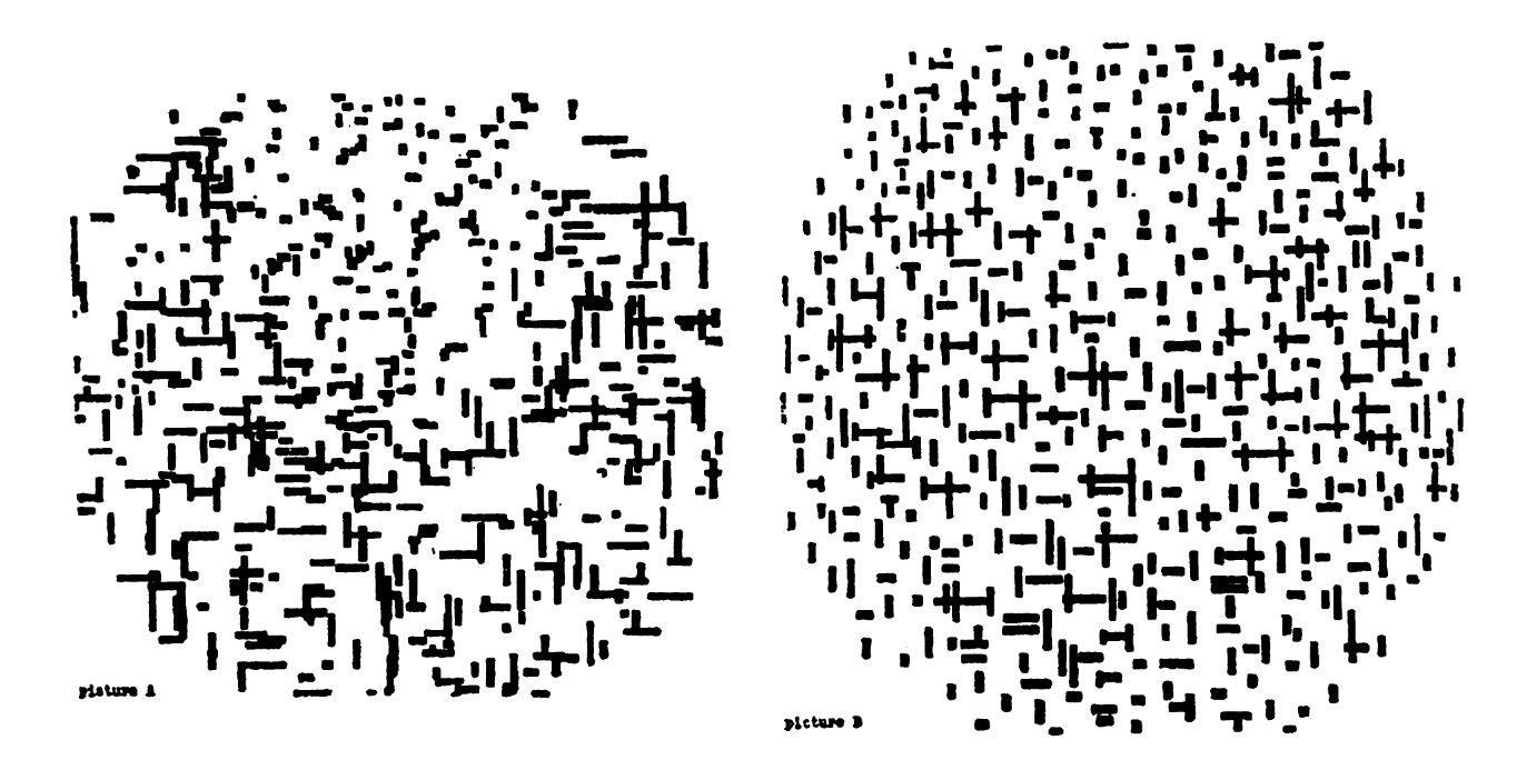
A. M. Noll, “Human or machine: A subjective comparison of piet mondrian’s”composition with lines” (1917) and a computer- generated picture,” The Psychological Record, vol. 16, pp. 1–10, 1966.

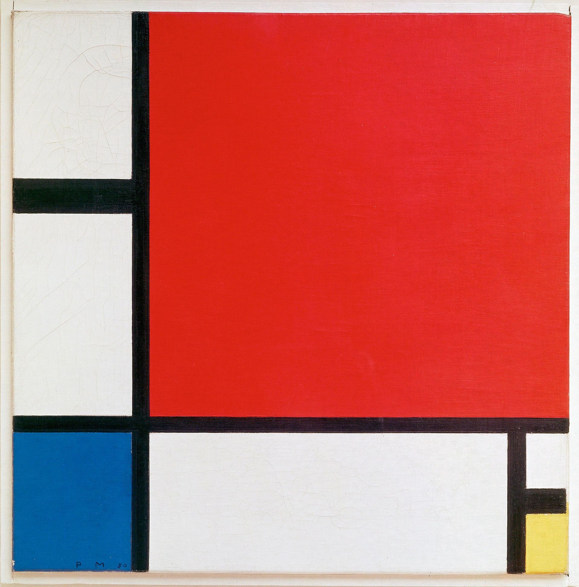
Aside: Who is Piet Mondrian?

Apophenia

What is apophenia?

The tendency to perceive a connection or meaningful pattern between unrelated or random things.

Visualization, statistical inference, visual inference

Visualization provides tools to uncover new relationships, tools of curiosity, and much of visualization research focuses on making the chance of finding relationships as high as possible
Statistical inference provides tools to check whether a relationship really exists (tools of skepticism) and most statistics research focuses on making sure to minimize the chance of finding a relationship that does not exist
- Testing: Is there a difference?
- Estimation: How big is the difference?
Visual inference bridges these two conflicting drives to provide a tool for skepticism that can be applied in a curiosity-driven context - Testing: Is what we see really there, i.e., is what we see in a plot of the sample an accurate reflection of the entire population?

Hypothesis testing as a court trial

Null hypothesis, $H_0$: Defendant is innocent
Alternative hypothesis, $H_A$: Defendant is guilty
Present the evidence: Collect data

Judge the evidence: “Could these data plausibly have happened by chance if the null hypothesis were true?”
- Yes: Fail to reject $H_0$
- No: Reject $H_0$

Hypothesis testing framework

Start with a null hypothesis, $H_0$, that represents the status quo
Set an alternative hypothesis, $H_A$, that represents the research question, i.e. what we’re testing for
Conduct a hypothesis test under the assumption that the null hypothesis is true and calculate a p-value (probability of observed or more extreme outcome given that the null hypothesis is true)
- if the test results suggest that the data do not provide convincing evidence for the alternative hypothesis, stick with the null hypothesis
- if they do, then reject the null hypothesis in favor of the alternative

Potential errors

Type 1 error (false negative): Acquit / reject $H_0$ when you shouldn’t
Type 2 error (false positive): Falsely convict an innocent / fail to reject $H_0$ when you shouldn’t
Costs of these errors vary based on the severity of the consequences

Statistical vs. visual inference

Statistical

Test statistic
p-value compared to significance level

Visual

Plot of the data
Humans’ picking an “innocent” out of a series of null plots

Visual inference with a lineup

The lineup protocol

Plot of the real data is randomly embedded amongst a set of null plots
Matrix of plots is known as a lineup
Null plots are generated by a method consistent with the null hypothesis
The lineup is shown to an observer. If the observer can pick the real data as different from the others, this puts weight on the statistical significance of the structure in the plot.
The lineup() function from the nullabor package returns a set of generated null datasets and the real data embedded randomly among these null datasets

Using `nullabor::lineup()`

Generating null plots:
- Option 1: Provide a method of generation and let the lineup() function generate them
- Option 2: Generating the null datasets yourself and pass them to the lineup() function

Position of the real dataset is hidden by default
- Decrypt to find out which plot is the real dataset

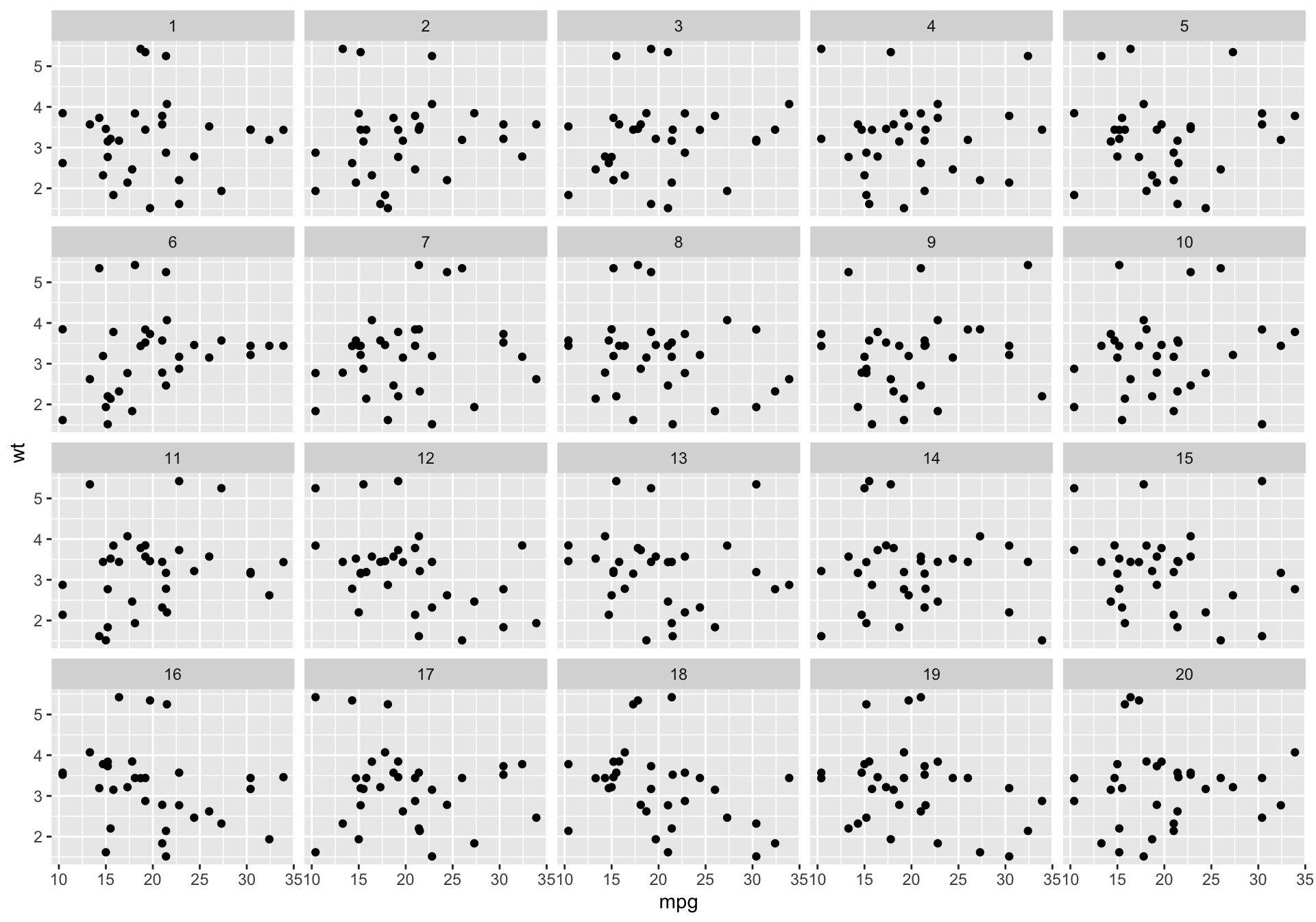
Will the real `mtcars` please stand up?

The making of the lineup I

Step 1. Permute the data

set.seed(20211029)
mtcars_permuted_lineup <- lineup(null_permute("mpg"), mtcars)

The making of the lineup II

Step 2. Peek at the permuted data

head(mtcars_permuted_lineup)

      mpg cyl disp  hp drat    wt  qsec vs am gear carb .sample
...1 10.4   6  160 110 3.90 2.620 16.46  0  1    4    4       1
...2 21.4   6  160 110 3.90 2.875 17.02  0  1    4    4       1
...3 14.7   4  108  93 3.85 2.320 18.61  1  1    4    1       1
...4 15.5   6  258 110 3.08 3.215 19.44  1  0    3    1       1
...5 30.4   8  360 175 3.15 3.440 17.02  0  0    3    2       1
...6 15.0   6  225 105 2.76 3.460 20.22  1  0    3    1       1

The making of the lineup II

Step 2. Peek at the permuted data

n = 20 by default

mtcars_permuted_lineup |>
  count(.sample)

   .sample  n
1        1 32
2        2 32
3        3 32
4        4 32
5        5 32
6        6 32
7        7 32
8        8 32
9        9 32
10      10 32
11      11 32
12      12 32
13      13 32
14      14 32
15      15 32
16      16 32
17      17 32
18      18 32
19      19 32
20      20 32

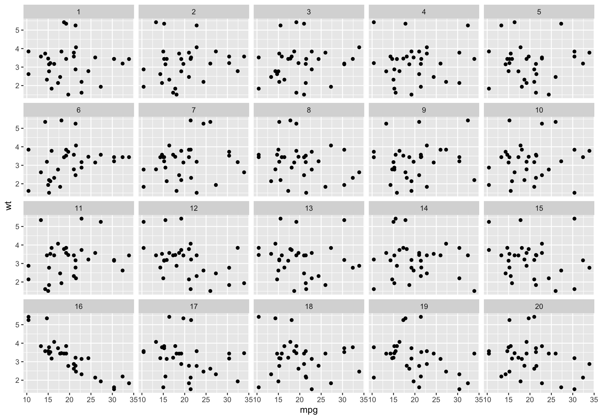
The making of the lineup III

Step 3. Plot the permutations

ggplot(data = mtcars_permuted_lineup, aes(x = mpg, y = wt)) +
  geom_point() +
  facet_wrap(~ .sample)

Decrypt the lineup

decrypt("K4Ul YG3G R8 oSJR3RS8 g6")

[1] "True data in position  16"

Visual inference with a Rorschach

The Rorschach protocol

The Rorschach protocol is used to calibrate the eyes for variation due to sampling
Plots generated corresponds to the null datasets, data that is consistent with a null hypothesis
rorschach() function returns a set of null plots which are shown to observers to calibrate their eyes with variation

Using `nullabor::rorschach()`

Generating null plots: Provide a method of generation and let the rorschach() function generate them
Provide the true data set
Set n, total number of samples to generate (n = 20 by default)
Set p, probability of including true data with null data (p = 0 by default)

Train your eyes to spot the real `mtcars`

The making of the rorschach I

Step 1. Permute the data

set.seed(20211029)
mtcars_permuted_rorschach <- rorschach(
  null_permute("mpg"), mtcars
)

The making of the rorschach II

Step 2. Peek at the permuted data

head(mtcars_permuted_rorschach)

   mpg cyl disp  hp drat    wt  qsec vs am gear carb .sample
1 10.4   6  160 110 3.90 2.620 16.46  0  1    4    4       1
2 21.4   6  160 110 3.90 2.875 17.02  0  1    4    4       1
3 14.7   4  108  93 3.85 2.320 18.61  1  1    4    1       1
4 15.5   6  258 110 3.08 3.215 19.44  1  0    3    1       1
5 30.4   8  360 175 3.15 3.440 17.02  0  0    3    2       1
6 15.0   6  225 105 2.76 3.460 20.22  1  0    3    1       1

The making of the rorschach II

Step 2. Peek at the permuted data

n = 20 by default

mtcars_permuted_rorschach |>
  count(.sample)

   .sample  n
1        1 32
2        2 32
3        3 32
4        4 32
5        5 32
6        6 32
7        7 32
8        8 32
9        9 32
10      10 32
11      11 32
12      12 32
13      13 32
14      14 32
15      15 32
16      16 32
17      17 32
18      18 32
19      19 32
20      20 32

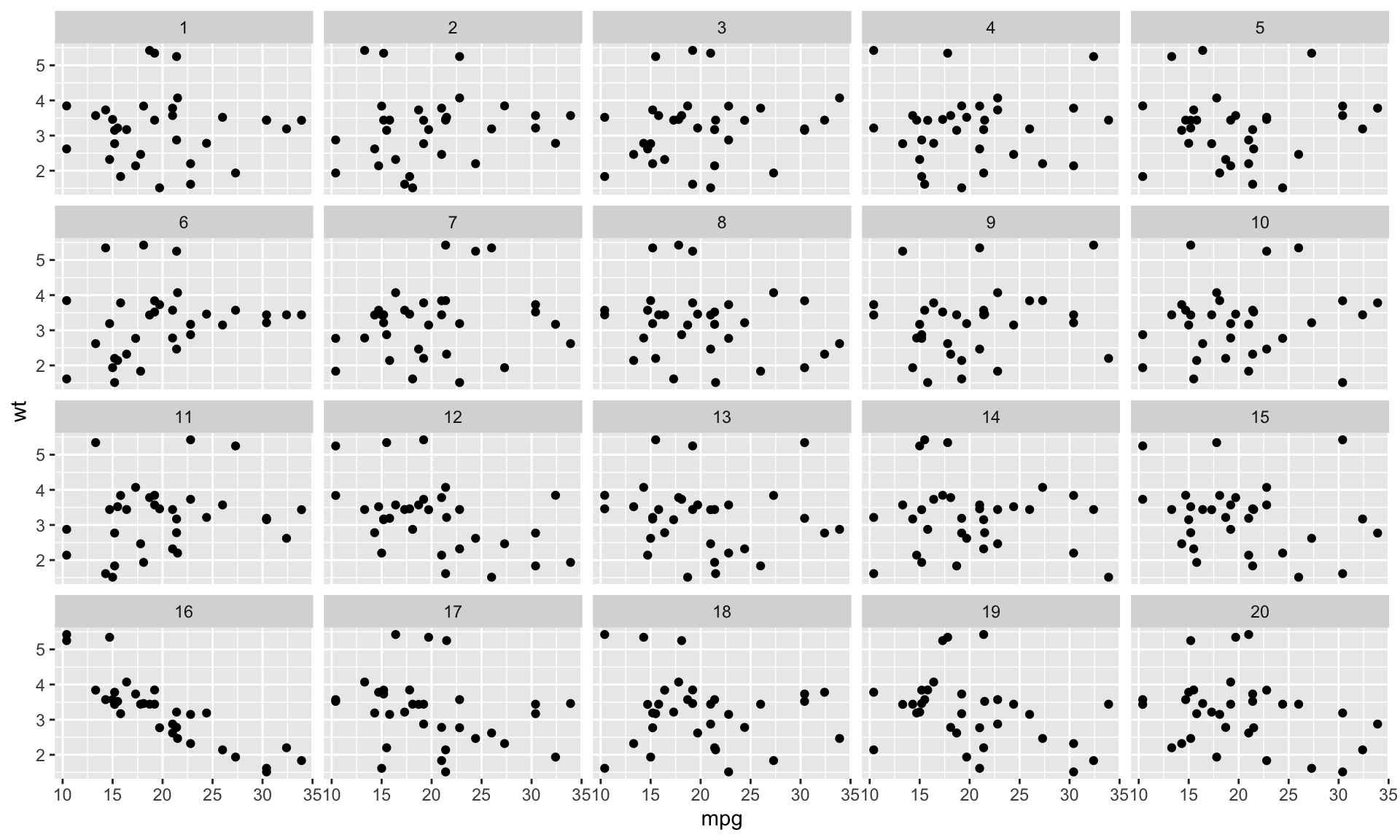
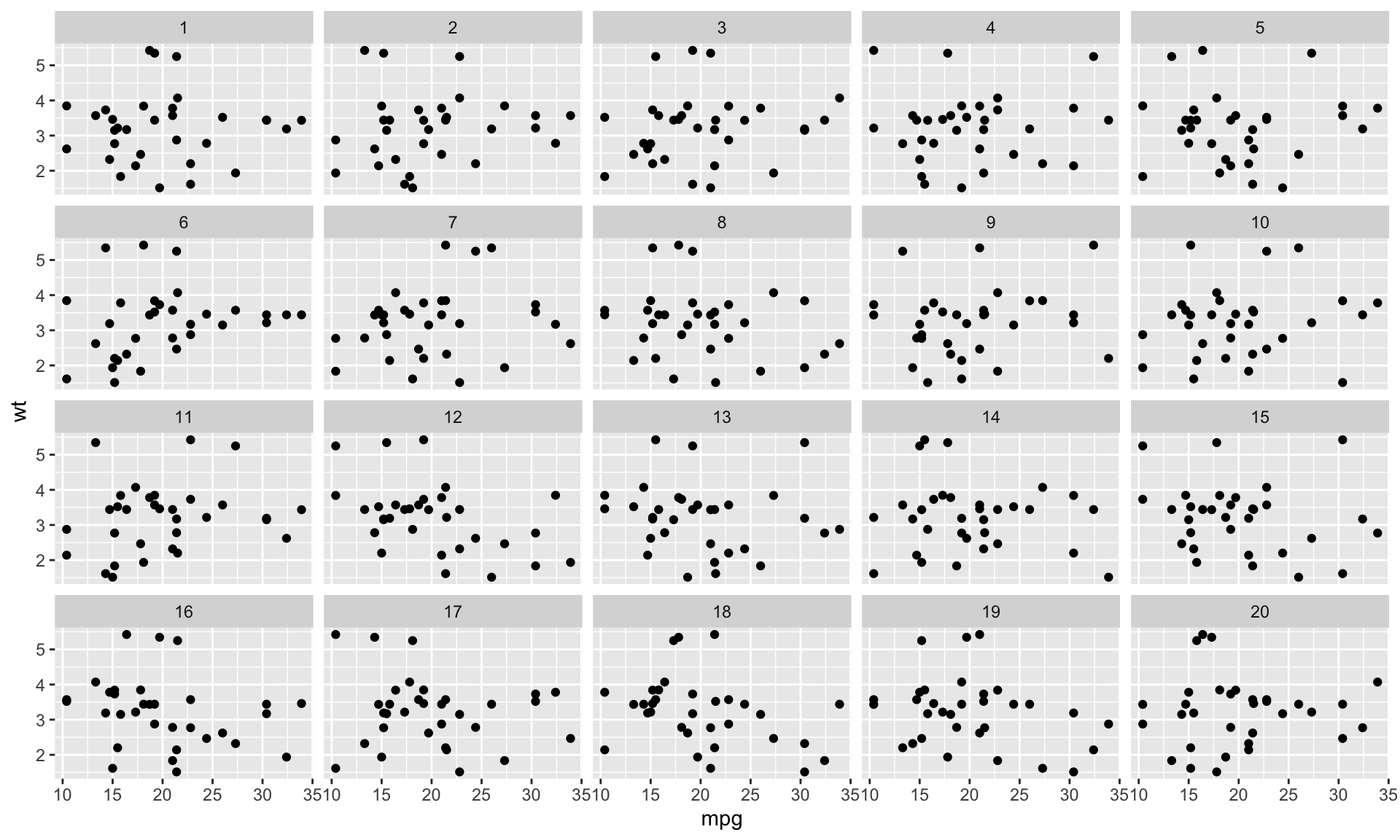
The making of the rorschach III

Step 3. Plot the permutations

ggplot(data = mtcars_permuted_rorschach, aes(x = mpg, y = wt)) +
  geom_point() +
  facet_wrap(~ .sample)

Decrypt the rorschach

In this particular case there’s nothing to decrypt since p (probability of including true data with null data) is set to 0
If p is higher than 0, and the true null is included, you get the decryption key

set.seed(12345)
mtcars_permuted_rorschach <- rorschach(null_permute("mpg"), mtcars, p = 0.5)
decrypt("K4Ul YG3G R8 oSJR3RS8 gI")

[1] "True data in position  15"

Generating the null data

By permuting a variable (what we’ve done so far with mtcars)
With a specific distribution
With null residuals from a model
With null data outside of nullabor (we won’t get into this, but see here for more)

Generate null data with a specific distribution

The null_dist() function takes as input a variable name of the data and a particular distribution
This variable in the data is substituted by random generations of the particular distribution
The different distributions include beta, cauchy, chi-squared, exponential, f, gamma, geometric, log-normal, lognormal, logistic, negative binomial, normal, poisson, t, and weibull
Parameters of the distributions are estimated from the given data (default) or can be provided as a list
null_dist() returns a function that generates a null data set given the data

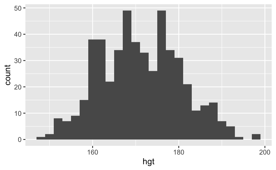
Case study: Heights of adults

The following histogram shows the distribution of heights of 507 physically active individuals (openintro::bdims$hgt). Do the heights of these individuals follow a normal distribution?

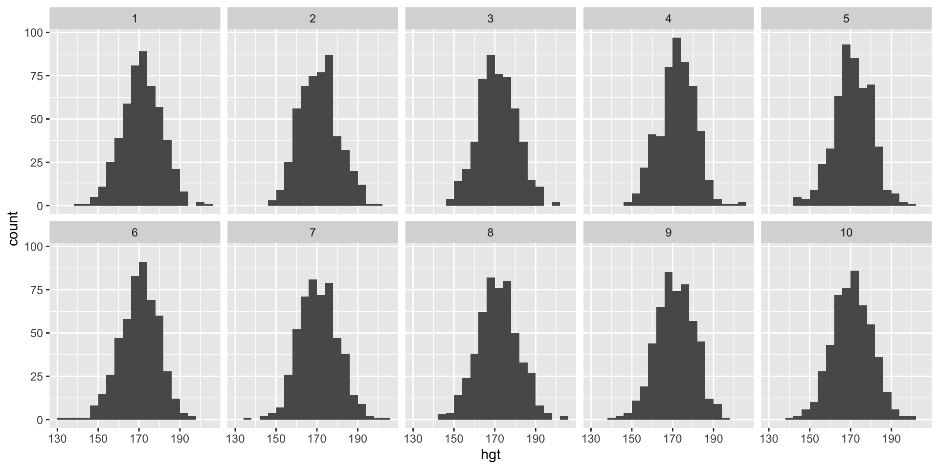
Spot the real data

Which of the following is the plot of the real data? (Note: A different binwidth than the previous plot is used.)

Code: Generate null data with a specific distribution

Generate the null distribution

set.seed(20211029)

bdims_permuted_lineup <- lineup(null_dist("hgt", dist = "normal"), n = 10, true = bdims)

Code: Decrypt

decrypt("K4Ul YG3G R8 oSJR3RS8 Ng")

[1] "True data in position  2"

Generating the null data with residuals from a model

null_lm() takes as input a model specification formula as defined by lm() and method for generating null residuals from the model
Three built in methods for different (and valid) methods to generate null data when fitting a linear model:
- method = "pboot"
- method = "boot"
- method = "rotate"
null_lm() returns a function which given the data generates a null dataset

Case study: Black cherry trees

Data measures the diameter, height and volume of timber in 31 felled black cherry trees (datasets::trees)

Summary

skim(datasets::trees)

── Data Summary ────────────────────────
                           Values         
Name                       datasets::trees
Number of rows             31             
Number of columns          3              
_______________________                   
Column type frequency:                    
  numeric                  3              
________________________                  
Group variables            None           

── Variable type: numeric ──────────────────────────────────────────────────────────────────────────────────────────────────────────────────────────────────────────────────────────────────────────────────────────────────────────────────────────────────────────────────────────────────────────────────
  skim_variable n_missing complete_rate mean    sd   p0  p25  p50  p75 p100 hist 
1 Girth                 0             1 13.2  3.14  8.3 11.0 12.9 15.2 20.6 ▃▇▃▅▁
2 Height                0             1 76    6.37 63   72   76   80   87   ▃▃▆▇▃
3 Volume                0             1 30.2 16.4  10.2 19.4 24.2 37.3 77   ▇▅▁▂▁

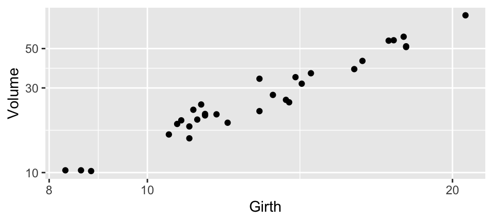
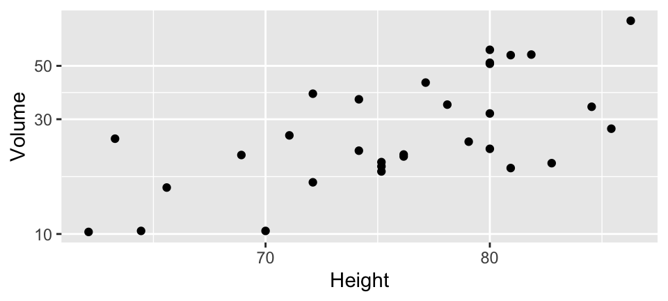
Case study: Black cherry trees

Plot

Fit the model

trees_fit <- lm(log(Volume) ~ log(Girth) + log(Height), 
                data = datasets::trees)

tidy(trees_fit)

# A tibble: 3 × 5
  term        estimate std.error statistic  p.value
  <chr>          <dbl>     <dbl>     <dbl>    <dbl>
1 (Intercept)    -6.63    0.800      -8.29 5.06e- 9
2 log(Girth)      1.98    0.0750     26.4  2.42e-21
3 log(Height)     1.12    0.204       5.46 7.81e- 6

Augment the model

trees_aug <- as_tibble(datasets::trees) |>
  mutate(
    .resid = residuals(trees_fit),
    .fitted = fitted(trees_fit)
  )

trees_aug

# A tibble: 31 × 5
   Girth Height Volume   .resid .fitted
   <dbl>  <dbl>  <dbl>    <dbl>   <dbl>
 1   8.3     70   10.3  0.0219     2.31
 2   8.6     65   10.3  0.0343     2.30
 3   8.8     63   10.2  0.0138     2.31
 4  10.5     72   16.4 -0.0106     2.81
 5  10.7     81   18.8 -0.0430     2.98
 6  10.8     83   19.7 -0.0420     3.02
 7  11       66   15.6 -0.0557     2.80
 8  11       75   18.2 -0.0443     2.95
 9  11.1     80   22.6  0.0822     3.04
10  11.2     75   19.9  0.00926    2.98
# ℹ 21 more rows

Test

Hypotheses:
- $H_0$: Errors are $NID(0, \sigma^2)$
- $H_A$: Errors are not $NID(0, \sigma^2)$

Visual statistic: Residuals plot (residuals vs. fitted)

Null distributions: Generate residuals from random draws from $N(0, \hat{sigma}^2)$ using the nullabor package

method <- null_lm(log(Volume) ~ log(Girth) + log(Height),
                  method = "pboot")

Compare the visual statistic from the data to the null distributions using a lineup

set.seed(2020)
trees_lineup <- lineup(method, true = trees_aug, n = 10)

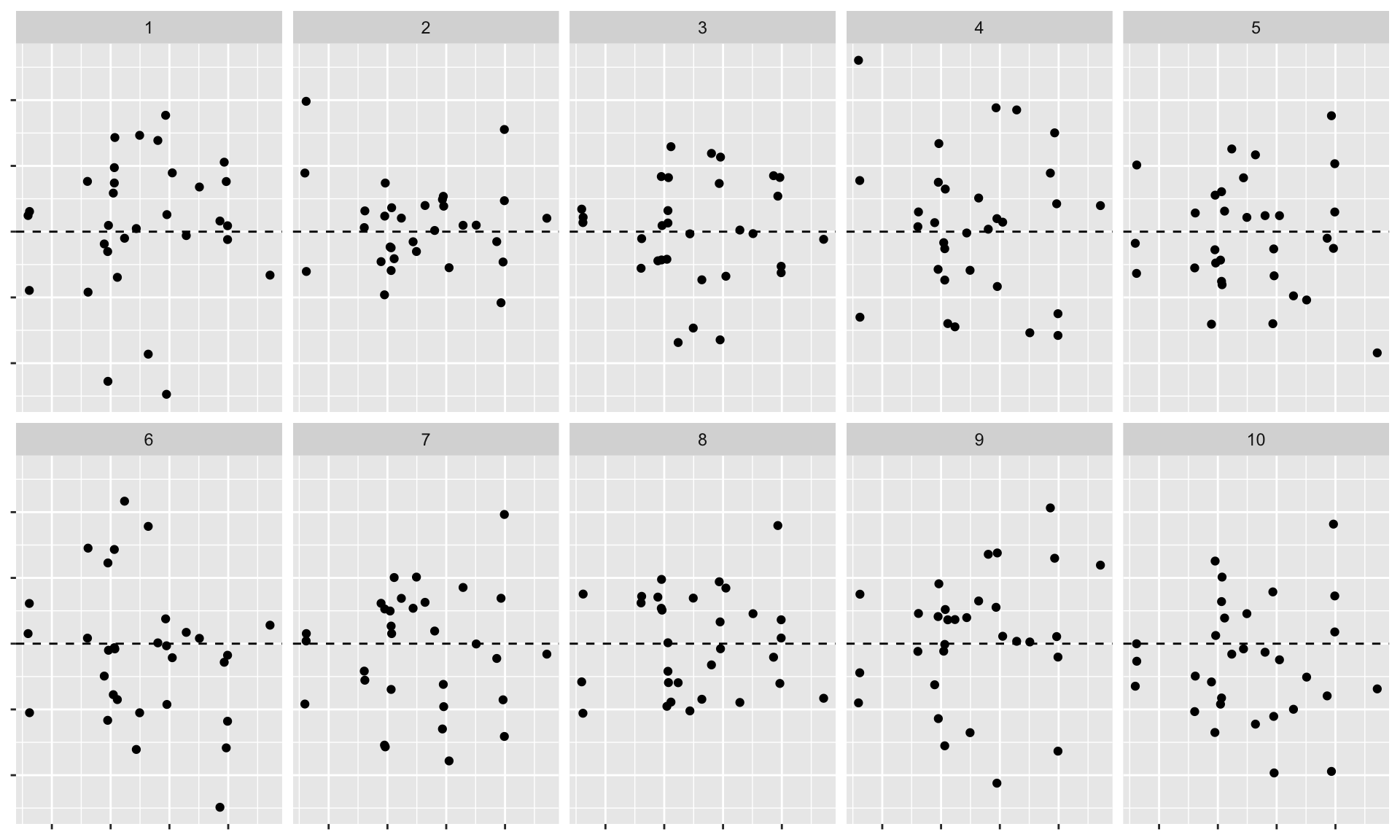
Lineup

Which one is the real residuals plot?

Decrypt

decrypt("K4Ul YG3G R8 oSJR3RS8 Nq")

[1] "True data in position  3"

The visual inference test

Notation:
- $n$: number of independent participants
- $X$: number of participants who detect the data plot
- $x$: observed value of $X$
- $m$: number of plots
- $p$: the probability of selecting the data plot

Hypotheses:
- $H_0: p = 1 / m$ - The probability of the data plot being selected is $1 / m$ (same as all other plots)
- $H_A: p > 1 / m$ - The probability of the data plot being selected is greater than $1 / m$

Under $H_0, X \sim B(n, 1/m)$. Then, visual inference p-value:

\[ p(X \ge x) = 1 - P(X \le x - 1) = \sum_{k = x}^n {n \choose k} \frac{(m - 1)^k}{m^n} \]

In R: $P(X \le x)$ = pbinom(x, n, p)

Calculating p-values

We did three lineup tests today, where - $x$ is the number of people who spotted the real data and - $n$ is the number of people voting

Let’s calculate the p-values

Spot the real mtcars (n = 20)

1 - pbinom(4, 12, 1/20)

Spot the real bdims::hgt (n = 10)

1 - pbinom(0, 12, 1/10)

Spot the real residuals of trees model (n = 10)

1 - pbinom(0, 12, 1/20)

Acknowledgements

Statistical inference for exploratory data analysis and model diagnostics by Andreas Buja , Dianne Cook , Heike Hofmann , Michael Lawrence , Eun-Kyung Lee , Deborah F. Swayne, and Hadley Wickham
Graphical Inference for Infovis by Hadley Wickham, Dianne Cook, Heike Hofmann, and Andreas Buja
Using computational tools to determine whether what is seen in the data can be assumed to apply more broadly by Emi Tanaka
Extending beyond the data, what can and cannot be inferred more generally, given the data collection by Emi Tanaka
The nullabor package

Visual inference

Warm-up

Announcements

Setup

Now you see me, now you don’t

Aside: Who is Piet Mondrian?

Apophenia

Visualization, statistical inference, visual inference

Hypothesis testing as a court trial

Hypothesis testing framework

Potential errors

Statistical vs. visual inference

Visual inference with a lineup

The lineup protocol

Using nullabor::lineup()

Will the real mtcars please stand up?

The making of the lineup I

The making of the lineup II

The making of the lineup II

The making of the lineup III

Decrypt the lineup

Visual inference with a Rorschach

The Rorschach protocol

Using nullabor::rorschach()

Train your eyes to spot the real mtcars

The making of the rorschach I

The making of the rorschach II

The making of the rorschach II

The making of the rorschach III

Decrypt the rorschach

Generating the null data

Generating the null data

Generate null data with a specific distribution

Case study: Heights of adults

Spot the real data

Code: Generate null data with a specific distribution

Code: Decrypt

Generating the null data with residuals from a model

Case study: Black cherry trees

Case study: Black cherry trees

Fit the model

Augment the model

Test

Lineup

Decrypt

The visual inference test

The visual inference test

Calculating p-values

Acknowledgements

Acknowledgements

Using `nullabor::lineup()`

Will the real `mtcars` please stand up?

Using `nullabor::rorschach()`

Train your eyes to spot the real `mtcars`