Modelling fish weights with multiple predictors

For this application exercise, we will continue to work with data on fish. The dataset we will use, called fish, is on two common fish species in fish market sales. We’re going to investigate the relationship between the weights and heights of fish, and later take into consider species as well.

library(tidyverse)
library(tidymodels)

fish <- read_csv("data/fish.csv")

The data dictionary is below:

variable	description
species	Species name of fish
weight	Weight, in grams
length_vertical	Vertical length, in cm
length_diagonal	Diagonal length, in cm
length_cross	Cross length, in cm
height	Height, in cm
width	Diagonal width, in cm

Interpreting multiple regression models

In the previous application exercise you saw that the model predicting weight from height and species was a better fit. In this section we will interpret the coefficients of this model.

fish_whs_fit <- linear_reg() |>
  fit(weight ~ height + species, data = fish)

tidy(fish_whs_fit)

# A tibble: 3 × 5
  term         estimate std.error statistic  p.value
  <chr>           <dbl>     <dbl>     <dbl>    <dbl>
1 (Intercept)    -828.      69.7     -11.9  1.92e-16
2 height           95.2      4.54     21.0  5.10e-27
3 speciesRoach    343.      41.8       8.19 6.35e-11

• What does each row in the model output represent?

The first row is the intercept. The second row is the slope for height. The third row is the slope for speciesRoach. In this case the other species level, Bream, is the reference level.

• Interpret the intercept and the slopes.

  • Intercept, -828: Bream fish that are 0 cm in height are expected to weigh, on average -828 grams. This value doesn’t make sense in context of the data.

  • height, 95.2: All else held constant, for each cm the height of fish is higher, weights of fish are expected, on average, to be higher by 95.2 grams.

  • speciesRoach, 343: All else held constant, Roach fish are expected, on averge to weigh 343 grams more than Bream fish, on average.

• Write the model.

\[ \widehat{weight} = -828 + 95.2 \times height + 343 \times speciesRoach \]

Additive vs. interaction models

• Run the two code chunks below and create two separate plots. How are the two plots different than each other? Which plot does the model we fit above represent?

ggplot(fish, aes(x = height, y = weight, color = species)) +
  geom_point(alpha = 0.5) +
  geom_smooth(method = "lm") +
  labs(title = "Plot A - Interaction model")

`geom_smooth()` using formula = 'y ~ x'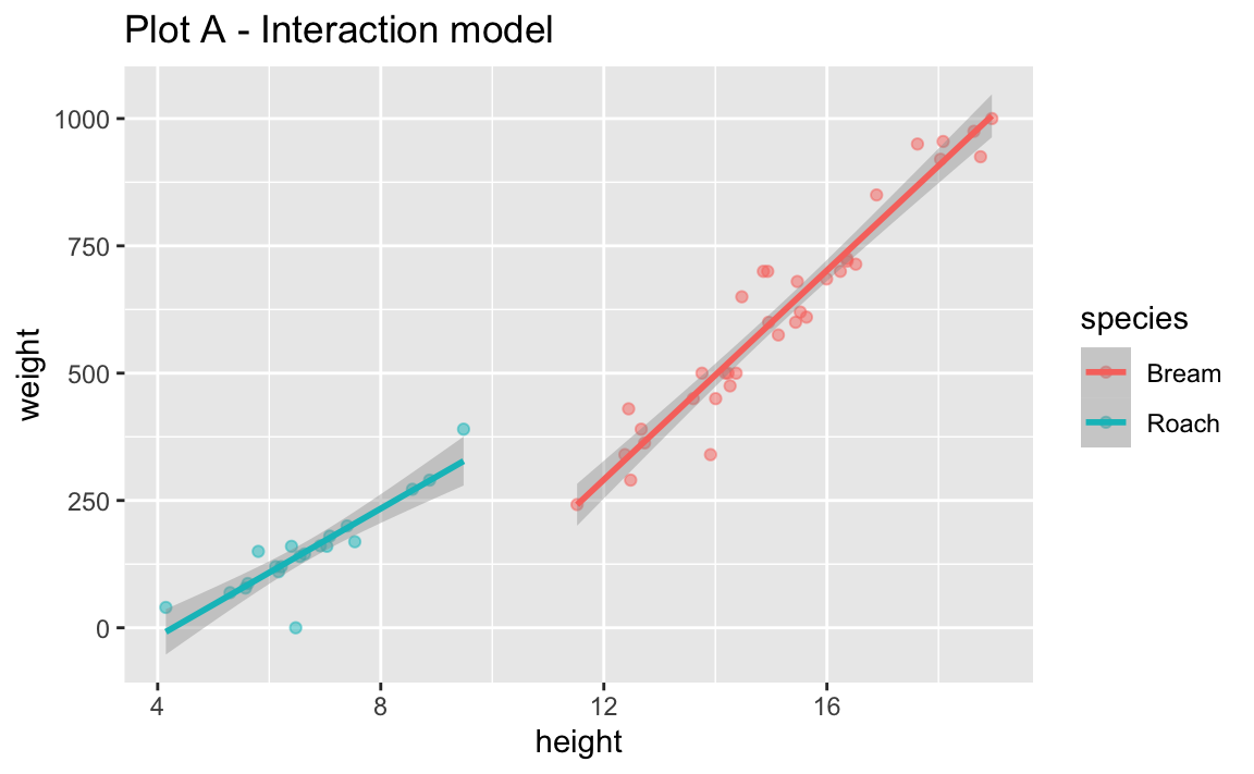

fish_whs_aug <- augment(fish_whs_fit, new_data = fish)

ggplot(
  fish_whs_aug, 
  aes(x = height, y = weight, color = species)
  ) +
  geom_point(alpha = 0.5) +
  geom_smooth(aes(y = .pred), method = "lm") +
  labs(title = "Plot B - Additive model")

`geom_smooth()` using formula = 'y ~ x'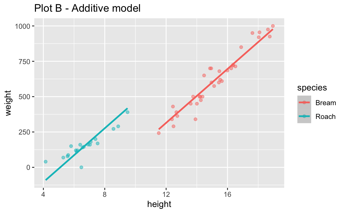

• Look back at Plot B. What assumption does the additive model make about the slopes between flipper length and body mass for each of the three islands?

The additive model assumes the same slope between height and weight of fish for the two species.

Choosing models

Rule of thumb: Occam’s Razor - Don’t overcomplicate the situation! We prefer the simplest best model.

• Choose a model using this principle.

# interaction

fish_whs_int_fit <- linear_reg() |>
  fit(weight ~ height * species, data = fish)

tidy(fish_whs_int_fit)

# A tibble: 4 × 5
  term                estimate std.error statistic  p.value
  <chr>                  <dbl>     <dbl>     <dbl>    <dbl>
1 (Intercept)           -942.      68.6     -13.7  9.20e-19
2 height                 103.       4.48     22.9  1.61e-28
3 speciesRoach           673.      93.5       7.20 2.64e- 9
4 height:speciesRoach    -39.9     10.4      -3.85 3.30e- 4

glance(fish_whs_int_fit)

# A tibble: 1 × 12
  r.squared adj.r.squared sigma statistic  p.value    df logLik   AIC   BIC
      <dbl>         <dbl> <dbl>     <dbl>    <dbl> <dbl>  <dbl> <dbl> <dbl>
1     0.969         0.968  51.3      540. 1.31e-38     3  -293.  595.  605.
# ℹ 3 more variables: deviance <dbl>, df.residual <int>, nobs <int>

# additive

fish_whs_fit <- linear_reg() |>
  fit(weight ~ height + species, data = fish)

tidy(fish_whs_fit)

# A tibble: 3 × 5
  term         estimate std.error statistic  p.value
  <chr>           <dbl>     <dbl>     <dbl>    <dbl>
1 (Intercept)    -828.      69.7     -11.9  1.92e-16
2 height           95.2      4.54     21.0  5.10e-27
3 speciesRoach    343.      41.8       8.19 6.35e-11

glance(fish_whs_fit)

# A tibble: 1 × 12
  r.squared adj.r.squared sigma statistic  p.value    df logLik   AIC   BIC
      <dbl>         <dbl> <dbl>     <dbl>    <dbl> <dbl>  <dbl> <dbl> <dbl>
1     0.961         0.959  57.7      634. 3.07e-37     2  -300.  607.  615.
# ℹ 3 more variables: deviance <dbl>, df.residual <int>, nobs <int>

Choose the interaction model since it has a higher adjusted R-squared.

• What is R-squared? What is adjusted R-squared?

R-squared is the percent variability in the response that is explained by our model. (Can use when models have same number of variables for model selection)

Adjusted R-squared is similar, but has a penalty for the number of variables in the model. (Should use for model selection when models have different numbers of variables).