Modelling fish weights with multiple predictors

For this application exercise, we will continue to work with data on fish. The dataset we will use, called fish, is on two common fish species in fish market sales. We’re going to investigate the relationship between the weights and heights of fish, and later take into consider species as well.

library(tidyverse)
library(tidymodels)

fish <- read_csv("data/fish.csv")

The data dictionary is below:

variable	description
species	Species name of fish
weight	Weight, in grams
length_vertical	Vertical length, in cm
length_diagonal	Diagonal length, in cm
length_cross	Cross length, in cm
height	Height, in cm
width	Diagonal width, in cm

Interpreting multiple regression models

In the previous application exercise you saw that the model predicting weight from height and species was a better fit. In this section we will interpret the coefficients of this model.

fish_whs_fit <- linear_reg() |>
  fit(weight ~ height + species, data = fish)

tidy(fish_whs_fit)

# A tibble: 3 × 5
  term         estimate std.error statistic  p.value
  <chr>           <dbl>     <dbl>     <dbl>    <dbl>
1 (Intercept)    -828.      69.7     -11.9  1.92e-16
2 height           95.2      4.54     21.0  5.10e-27
3 speciesRoach    343.      41.8       8.19 6.35e-11

• What does each row in the model output represent?

Add response here.

• Interpret the intercept and the slopes.

Add response here.

• Write the model.

Add response here.

Additive vs. interaction models

• Run the two code chunks below and create two separate plots. How are the two plots different than each other? Which plot does the model we fit above represent?

ggplot(fish, aes(x = height, y = weight, color = species)) +
  geom_point(alpha = 0.5) +
  geom_smooth(method = "lm", se = FALSE) +
  labs(title = "Plot A - Interaction model")

`geom_smooth()` using formula = 'y ~ x'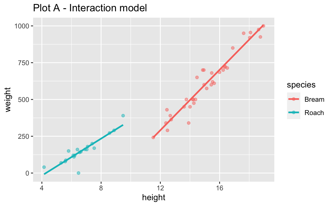

fish_whs_aug <- augment(fish_whs_fit, new_data = fish)

ggplot(
  fish_whs_aug, 
  aes(x = height, y = weight, color = species)
  ) +
  geom_point(alpha = 0.5) +
  geom_smooth(aes(y = .pred), method = "lm", se = FALSE) +
  labs(title = "Plot B - Additive model")

`geom_smooth()` using formula = 'y ~ x'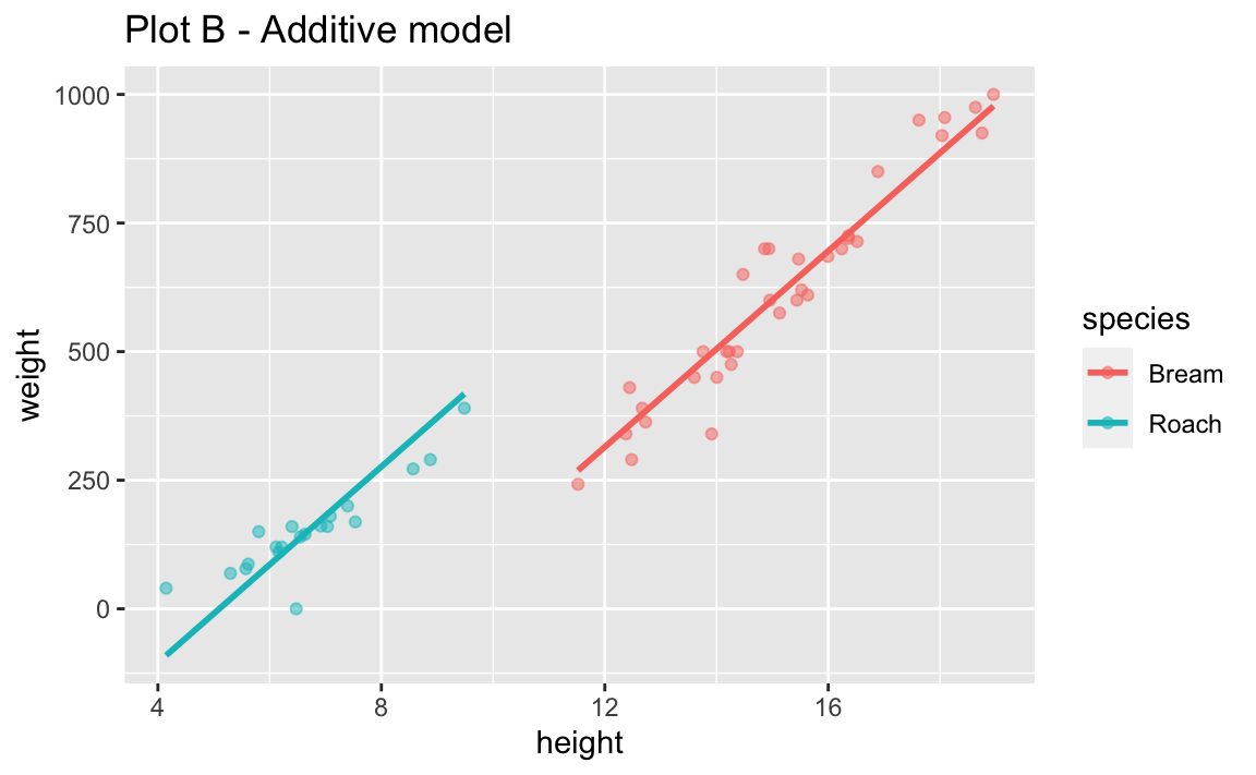

• Look back at Plot B. What assumption does the additive model make about the slopes between flipper length and body mass for each of the three islands?

Add response here.

Choosing models

Rule of thumb: Occam’s Razor - Don’t overcomplicate the situation! We prefer the simplest best model.

• Choose a model using this principle.

# add code here

Add response here.

• What is R-squared? What is adjusted R-squared?

Add response here.